Module 5: Building species trees
Phylogenetic species trees are diagrams that represent the evolutionary relationships between different species. They depict the branching patterns and common ancestry among species, providing a visual representation of their evolutionary history. Species trees are useful because they provide insights into the origin, divergence, and relationships between species, allowing us to study their evolutionary history.
The accuracy of the species tree is important for OMA because it is needed to construct HOGs at each taxonomic level. If the species tree is incorrect or unresolved, the quality of HOG inference at certain taxonomic levels will be affected.
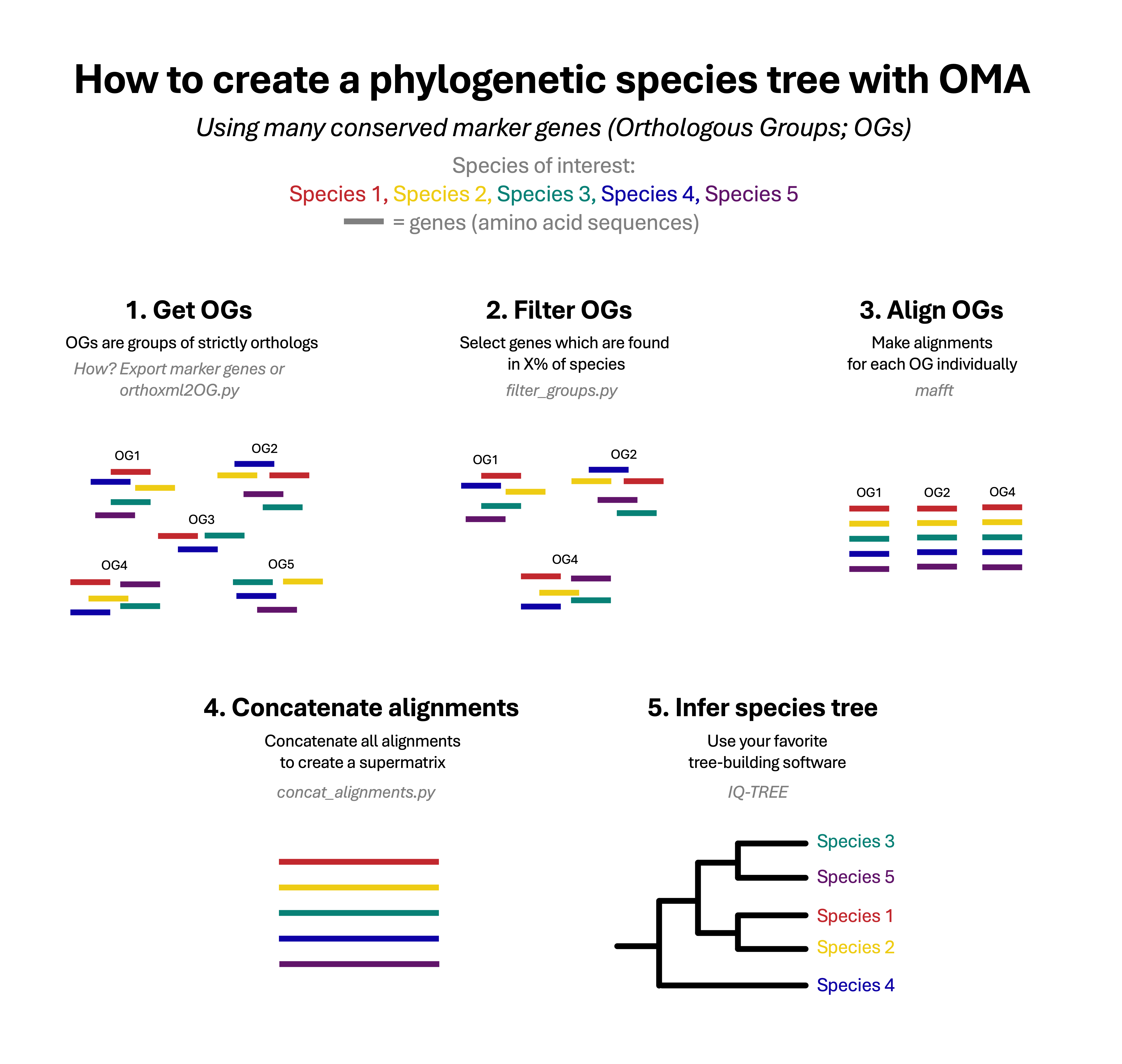
A commonly used method to create a phylogenetic species tree is by using multiple protein-coding genes that are conserved across multiple species. This method involves several steps: orthology inference, multiple sequence alignment, and construction of the phylogeny with dedicated software.
This module was created based on the tutorial “How to build phylogenetic species trees with OMA” by Dylus et al, published in F1000’s OMA Collection.
5.1. Retrieving marker genes from selected species
Depending on which species you want to make a species tree for, two options are available to obtain OG data:
- Do you want to make a phylogeny with species that are all found in the OMA Browser?
- With your own species, preprocessed using FastOMA (see Module 3)?
Go to which option to follow: Module 5.1.1 to use only precomputed groups with species available on the OMA Browser.
Optional Go to Module 5.1.2, Computing Orthologous Groups using the output of FastOMA.
5.1.1. Make a tree with species that can be found in the OMA browser
- Saccharomyces cerevisiae (strain ATCC 204508 / S288c)
- Schizosaccharomyces pombe (strain 972 / ATCC 24843)
- Sclerotinia sclerotiorum (strain ATCC 18683 / 1980 / Ss-1)
- Yarrowia lipolytica (strain CLIB 122 / E 150)
- Neosartorya fumigata (strain ATCC MYA-4609 / Af293 / CBS 101355 / FGSC A1100)
Remember, we want OGs that are present in the majority of the species of interest. How to get this? In the OMA browser, go to Download-> Export Marker Genes and search for the species.
- Select all species: A whole clade can be selected by clicking on the node and clicking “select all species.”
- Select a single species: A single species can be selected by clicking on the leaf and clicking “select species.”
- Display a clade’s name: A whole clade can be collapsed by clicking on the node and selecting “collapse all.” Collapsing all the nodes in a clade will display the clade’s name.
1. In which clade was their last common ancestor?
Ascomycota2. Out of the 5 species, which one is the outgroup?
Schizosaccharomyces pombe
After selecting your genomes, you can vary two parameters for this step:
- Maximum nr of markers: the number of genes you wish to export via the OMA browser (too many increases the required computation)
- Minimum fraction of covered species: the proportion of species that must be in a group
The goal is to have enough conserved genes (OGs) to amplify the phylogenetic signal but not too much as to use too many computational resources. As a rule of thumb, the best is to have between 100 and 1000 genes.
Set 1.0 as the proportion of species and set the number of genes to -1 (no limit). Click Submit to export the marker genes and download the resulting compressed file. This should take a few minutes.
wget <URL comes here>” .
3. What types of files are found in the output?
FASTA files, both amino acid and nucleotide sequences
We need to adjust the file headers so that the name of the species is shorter, and with underscores instead of spaces. This will come in handy down the line when we make the tree and visualize it, because spaces in labels can cause compatibility issues in the output files. Run the following command to edit the headers in each amino acid fasta file.
for file in marker_genes/*.fa; do
    sed 's/\[Saccharomyces cerevisiae (strain ATCC 204508 \/ S288c)\]/\[Saccharomyces_cerevisiae\]/g' "$file" > "$file.tmp"
    sed 's/\[Schizosaccharomyces pombe (strain 972 \/ ATCC 24843)\]/\[Schizosaccharomyces_pombe\]/g' "$file.tmp" > "$file.tmp2"
    sed 's/\[Sclerotinia sclerotiorum (strain ATCC 18683 \/ 1980 \/ Ss-1)\]/\[Sclerotinia_sclerotiorum\]/g' "$file.tmp2" > "$file.tmp3"
    sed 's/\[Yarrowia lipolytica (strain CLIB 122 \/ E 150)\]/\[Yarrowia_lipolytica\]/g' "$file.tmp3" > "$file.tmp4"
    sed 's/\[Neosartorya fumigata (strain ATCC MYA-4609 \/ Af293 \/ CBS 101355 \/ FGSC A1100)\]/\[Neosartorya_fumigata\]/g' "$file.tmp4" > "$file.tmp5"
    mv "$file.tmp5" "$file"
    rm "$file.tmp" "$file.tmp2" "$file.tmp3" "$file.tmp4"
done
The headers should now be in the format of: >ASPFU03763 | OMA969106 | E9RB80 | [Neosartorya_fumigata]
5.1.2. Make a tree using FastOMA results (Optional)
You might wish to make a species tree using your own custom genomes. In this case, you would use the Orthologous Groups inferred with FastOMA as marker genes to then create a species tree. This species tree can then be reused in FastOMA to further refine the HOG inference.
When running FastOMA, always make sure to include an outgroup; that is a species you know is more distantly related than all the others.
The output of FastOMA includes a folder named OrthologousGroupsFasta (compressed files).
Note that the answers in the rest of this module are designed based on the result of the OMA browser (Section 4.1.1) and will vary slightly from the answers using the FastOMA results. However, the major steps in the tutorial remain the same.
5.2. Filter Orthologous Groups
We now need to filter the OGs based on the number of species present in them in order to get the correct number of Orthologous Groups, and/or to get the header in the correct format.
To do this, we will use a python script available in the Dessimoz Lab GitHub. This, and other python scripts we will use later in the Module, should already be installed on the GitPod in the folder f1000_PhylogeneticTree.
Optional: Download the git repo with the following command: git clone https://github.com/DessimozLab/f1000_PhylogeneticTree.git
Then, execute the following command to filter OGs:
python f1000_PhylogeneticTree/filter_groups.py -n 5 -i marker_genes -o filteredOGs
Here the parameter “n” specifies the minimum number of species we want included in each Orthologous Group (here we chose 5, because we think we can find sufficient Orthologous Groups with sequences from all 5 species).
Note: If you obtained the OGs from step 4.1.1 (species coverage parameter set to 1.0), then filtering with -n 5 would be optional. However, in this example, it is important to connect with the next steps.
1. How many groups of genes do you have?
find filteredOGs/ -type f -name "*.fa" | wc -l977
5.3. Create supermatrix
We will create a species phylogeny by aligning all the sequences within each orthologous group and then combining these alignments into a single concatenated alignment: this is called a supermatrix. It is then used as input to tree estimation software to obtain the species tree.
mkdir alignments
cd filteredOGs
for i in $(ls -1 *.fa | head -100); do
    if [ ! -s $i.aln ]; then
        mafft --maxiterate 1000 --localpair $i > ../alignments/$i.aln 2>>../align.log;
    fi
done
cd ..
1. How would you adapt the code to align the 200 first maker genes?
Replacehead -100byhead -200in the for-loop.2. Open up one of the alignment files. What format are these alignments in?
cd /workspace/SIBBiodiversityBioinformatics2023/Module4_SpeciesTrees/working_dir/alignments/
cat <OMAGroup_X>.fa.aln>
FASTA format
The next step is to concatenate the alignments into the supermatrix. A Python script from the f1000_PhylogeneticTree (concat_alignments.py) is available to perform this. It can be run as so:
python f1000_PhylogeneticTree/concat_alignments.py alignments/*aln --format-output fasta > supermatrix.aln
3. What size is the new, concatenated alignment (how many rows and how many columns)?
The number of columns in the supermatrix are the number of amino acids in the alignment. The number of rows is the number of species, which can be counted using the sequence headers in a fasta-formatted file with the commandgrep -c ">" supermatrix.aln. Use the following command to find the number of amino acids:grep -v '^>' supermatrix.aln | tr -d '\n' | wc -mThe concatenated supermatrix is 298550 positions long, for 5 species (numbers might slightly change by run).
5.4. Build a species tree
Finally, we will use phylogenetic software to estimate the species tree. Here, we propose using IQ-TREE, which is a method to create maximum likelihood (ML) trees. A maximum likelihood tree is constructed with the goal to find the tree topology and branch lengths that maximize the likelihood of observing the given sequence data under a specific evolutionary model.
iqtree -s supermatrix.aln -B 1000 -T 8 -mset WAG,LG
- iqtree: This is the command to invoke the IQ-TREE program.
- -s all_concat_OGs.aln: This option specifies the input multiple sequence alignment (MSA) file. In this case, the file named all_concat_OGs.aln contains the aligned sequences that will be used to build the phylogenetic tree.
- -B 1000: This option specifies the number of ultrafast bootstrap replicates for assessing branch support. In this case, the value is set to 1000, indicating that IQ-TREE will perform a non-parametric bootstrap analysis with 1000 replicates to estimate branch support values
- -T 8: This option specifies the number of threads (CPU cores) to use for parallel computation. In this example, IQ-TREE will use 8 threads to speed up the analysis. Note that in the GitPod workspace, you likely have only 4-8 CPUs.
- -mset WAG,LG restricts the model search to models based on the WAG and LG amino/acid substitution matrices. This is to avoid spending too much time searching through many different evolutionary models, which is not needed for a tree as simple as the one we are computing here.
We have provided the results of the IQ-TREE run in the expected_out folder (cp ../expected_output.iqtree.tar.gz to copy it to your working directory and also available online here). However, note that if running yourself, you will likely need to perform on an HPC, especially if you have many species you wish to construct a tree for. Large trees could take up to 50 GB of RAM. An example of a slurm job script to run IQ-TREE can be found here.
#!/bin/bash
#SBATCH --partition=cpu
#SBATCH --nodes=1
#SBATCH --ntasks=1
#SBATCH --cpus-per-task=45
#SBATCH --time=50:00:00
#SBATCH --mem=50GB
#SBATCH --job-name=iqtree
#SBATCH --output=logs/iqtree-%J.log
#SBATCH --export=None
#SBATCH --error=logs/iqtree-%J.err

module load gcc/10.4.0
module load iq-tree/2.2.0.5-openmp

mkdir logs
iqtree -s supermatrix.aln -B 1000 -T 45
1. How long did the job take?
Look in the IQ-TREE log file.Total CPU time used: 456.538 sec (0h:7m:36s)
Total wall-clock time used: 126.231 sec (0h:2m:6s)Note: These values are accurate for the iqtree log file provided in the expected output folder (4.1.1). This answer may vary depending on the number of CPUs available.
When constructing a maximum likelihood tree, it performs a model selection as the first step. That is, it chooses an appropriate evolutionary model that describes the substitution patterns (mutations). Different models account for different types of evolutionary processes, such as transitions, transversions, and rate heterogeneity.
2. Which model did the ModelFinder find as the best fit and why?
Best-fit model: LG+F+I+G4 chosen according to BIC (Bayesian information criterion).
5.5. Evaluating the species tree
Once a phylogeny has been obtained, it is important to have the tools to visualise it and help interpret it. Particularly because, even if they are displayed in an unambiguous way, uncertainty may exist in the topology.
For this section, we will use the tree you obtained in the last module. If you skipped this part, please use the IQ-TREE tree available in the expected_output folder for this module in GitPod (cp ../expected_output.iqtree.tar.gz to copy it to your working directory or available online here.
Upload your newick file of the ML tree to the online tree visualizer, phylo.io. It can be found as the “.treefile” in the IQ-TREE results.
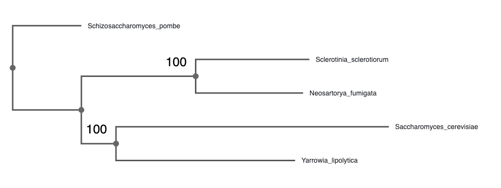
Reroot the tree based on the outgroup sequences you included earlier (section 5.1.1).
1. Which species is most closely related to Saccharomyces cerevisiae?
Click on the branch and click “Reroot”Yarrowia lipolytica
Now, examine the bootstrap values. Click on Settings -> Branches and Levels -> Data to display the ultrafast bootstrap values.
2. Which clades can be considered well supported by the data?
According to the IQ-TREE documentation, 95 is a commonly accepted threshold for ultrafast bootstrap values, as it roughly corresponds to a 95% probability that the clade is correct.Both the (S. cerevisiae, Y. lipolytica) and the (S. sclerotiorum, N. fumigata) clades are supported with 100% ultrafast bootstrap support. (Note that the branch lengths may be slightly different than shown here.)